In the following article, we will discuss about the Naive Bayes classification algorithm, its mathematical representational and we will train a model on Python that predicts news categories given news titles.

Most cases of classification in language processing are done via supervised machine learning, that is a process where we have a data set of input observations associated with some correct output, called a supervision signal. The goal of any classification algorithm is to learn how to map from a new observation to a correct input.

The task of a classification algorithm is to take a set of inputs x and a set of output classes Y, and return a predicted class y ∈ Y. For text classification, it’s common to see inputs x being referred with the letter d for “documents” and outputs Y as c for “classes”, and that is how we will be referring to them today as well. Words in documents are often referred to as “features”.

There are many algorithms that are used to build classifiers, but as stated above, the one we will be working with is the Naïve Bayes algorithm.The latter, also has many variants depending on the type of features and classes. The one that is fit for our classification purposes is the Multinomial type.

NB is a probabilistic classifier, which tells us the probability of the observation being in the class. What that means for our case is that for each feature with class c, we will calculate the probability using a formula, which I will get to in a second, and in the end we will pick the highest probability, which evaluates to a class.

The initial formula is this:

Prior probability P(c) is calculated as the percentage of documents in our training data that are in class c.

Where Nc is the total number of documents with class c in our data, and Ndoc is the total number of documents.

Since document d is represented as a set of features (words) w, the initial likelihood formula per word in a class is:

Which means the likelihood equals a fraction between the count of the given word w-i in the class c and the count of all words w in the class c.

This, however has a flaw. If we are computing probability for a word which is in our vocabulary V but not in a specific class, the probability for that pair will be 0. But since we multiply all feature likelihoods together, zero probabilities will cause the probability of the entire class to be zero as well. For this we need to add a smoothing technique. Smoothing techniques are popular in the language processing algorithms. Without getting too much into them, the technique we will be using is the Laplace one which consists in adding + 1 to our calculations. The formula will end up looking like this:

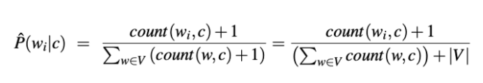
Where V is a collection of our word types. Word types is a list of unique words we have in our documents.

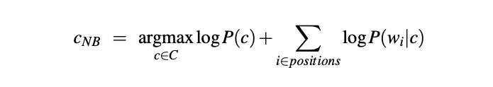
We have to note that the language processing calculations are done in log space to avoid underflow and increase speed. Naïve Bayes algorithm is no different from that. As such, the first formula evaluates to:

Now to the fun part,

Native implementation of Multinomial Naïve Bayes algorithm in Python

Naïve Bayes algorithm is a popular classification algorithm and as such has support through some different packages — see section “Alternative approach”. However, in our implementation we will be taking a completely native approach. The goal of this project is to implement the algorithm to make a prediction on a news category if we type in the news title.

Prerequisites

We will be developing our script in a Python 3.x environment. We will be making use of Numpy package for our array operations and Pandas for managing our data. Speaking of which, the use of data will be explained in the upcoming section — “Working with data”.

Training

Training / building / fitting a ML model means using some set of data to generate information which we will then use to make our predictions. Depending on the purpose, the training method is meant to implement the ML algorithm and that can be from easy to complex. In our case, the method will implement the formulas we have described above and will generate the necessary data for making the predictions such as probabilities, likelihoods and vocabularies.

The training will be done inside a method we’re calling fit().

In our fit method we assume that documents and classes are given in two separate vectors that maintain their relationship via indexes. In this method we also generate vocabularies.

Building the vocabulary

In our algorithm, we will need two kinds of vocabularies. One is a list of all unique word types which we will call global vocabulary, and the other one is a class specific vocabulary, containing words of documents for each class organised in a dictionary.

The implementation of methods for generating the respective vocabularies is:

As you can see, in those methods we have used a custom method cleanDoc which processes each document. Now, in the language processing algorithm, a cleaning method might include operations to remove things such as stop words like the and a which can be common but in our case removing the stop words doesn’t improve performance and as such the only cleaning we will do is strip the document away from punctuation, lowercase the letters and split it by space.

In the fit method, we get a unique list of items from our classes list. Then we iterate that list and for each unique class we generate logprior, build the class vocabulary, and for each word in the global vocabulary list, we basically check the counter in the current class and in the vocabulary. Inside the word iteration we resolve the loglikehood for the word-class pair.

We keep information such as logprior, class vocab and loglikehood in dictionaries. To get counts for words, we use the Counter collection.

The entire fit() method looks like this:

Testing

Testing / predicting methods contain an algorithm that evaluates the model we have trained. In our case, for each unique class and for each word in a testing document, we look for previous probabilities of such pairing and add it to a total sum of that class’ probability, which is initialised with the logprior value of that class. In the end, we get the maximum value from all the sums and eventually we narrow it down to a class.

We have fit this logic under the predict method.

Working with data

Finding (and generating) a good dataset for data analyzing purposes is a discipline on its own. The dataset can be disbalanced, you can have too much data, or too little data. You can overfit or underfit data. In this article, we won’t be pre-processing our data, at least not a lot.

For our goal, we will use the News Aggregator dataset, which was generated by the UCI over the dates of March 10th, 2014 to August 10th, 2014. This dataset contains around 400k lines of news split into several columns, including title and category. Each news item belongs to one of the four categories: “Business”, “Science and Technology”, “Entertainment”, “Health” labeled as b, t, e, m respectively.

We will be using Pandas to read our data. We will be also splitting the dataset into training and testing data. We will be customising our reader method to accept arguments on the size of data we will read and the split ratio.

Putting it all together

In the main method, we put all things together. Get the data, train our classifier and test it using our test data. In the end, we measure the accuracy score.

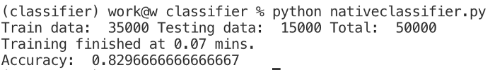
In the model that we have trained with 35000 documents, and tested on 15000 other documents we have achieved a 82.9% accuracy score, which is a very good one.

To avoid having to train the model every time we want to make a prediction, we can pickle the generated data. The helper methods for doing that are:

And the entire fit and predict methods are changed as follows:

And their implementation has changed to:

This way we have build a model that is able to make predictions on what news category, a news title belongs to. The full code can be found here.

Alternative approach

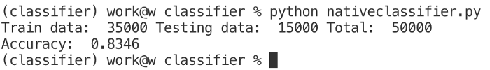
As pointed out above, the Naïve Bayes is a popular classification algorithm and as such is supported by several packages. One of the most popular is Sklearn. It offers support for all types of Naïve Bayes classification. When working with the multinomial one, input is transformed with CountVectorizer, which is a data encoder, and that results in faster training and testing times. Accuracy, however, is only slightly higher than with our natively implemented algorithm, at 83.4% using the same training and testing data as before.

References:
1. Jurafsky, Dan & Martin, James. Speech and Language Processing.
2. Lichman, M. (2013). UCI Machine Learning Repository [http://archive.ics.uci.edu/ml]. Irvine, CA: University of California, School of Information and Computer Science.